Tutorial: Sampler comparison

This tutorial demonstrates the difference between the Random sampler and the Grid sampler over a 2D parameter space. The runner implements a synthetic test funtion consisting of two Gaussian peaks with a background slope (Synthetic Double Gaussian Runner). The function implemented in the runner (with default parameters) looks like this:

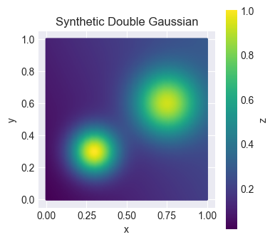
The function symbolizes an unknown sample space that we want to try to represent by drawing samples using different strategies.

Run the example

Setup two new configuration files based on configs/example_local.yaml.

cd enchanted-surrogates/
cp configs/example_local.yaml configs/example_local_random.yaml
cp configs/example_local.yaml configs/example_local_grid.yaml   

Edit example_local_random.yaml to have parameters:

samplers:
  s1:
    type: RandomSampler
    bounds: [[0.0, 1.0], [0.0, 1.0]]
    budget: 100
    parameters: ['x', 'y']

...

supervisor:
  base_run_dir: "data_dir/local_random"
  ...

Edit example_local_grid.yaml to have parameters:

samplers:
  s1:
    type: GridSampler
    bounds: [[0.0, 1.0], [0.0, 1.0]]
    num_samples: [10, 10]
    parameters: ['x', 'y']

...

supervisor:
  base_run_dir: "data_dir/local_grid"
  ...

In the random sampler, the budget defined the total number of samples. In the grid sampler, the num_samples defiend how many samples per parameter. The total number of samples is the product of all values in num_samples. In this case 10*10=100. The same number of samples have been configured for both cases. The same parameters and parameters bounds have also been configured for both cases.

Run enchanted-surrogates with the new configs.

python src/run.py -cf configs/example_local_random.yaml

python src/run.py -cf configs/example_local_grid.yaml

This will create two separate directories, both containing 100 samples over the same parameter space but distributed differently.

Results

Now we can take a look at the generated samples by reading the summary files enchanted_dataset.csv.

import matplotlib.pyplot as plt
import matplotlib as mpl
import pandas as pd

# Read summary files csv
csv_path_grid = "data_dir/local_grid/enchanted_dataset.csv"
if os.path.exists(csv_path_grid):
    df_grid = pd.read_csv(csv_path_grid)

csv_path_random = "data_dir/local_random/enchanted_dataset.csv"
if os.path.exists(csv_path_random):
    df_random = pd.read_csv(csv_path_random)

fig, axs = plt.subplots(1, 2, figsize=(10, 4))

# Shared colorbar
vmin = min(df_grid['output'].min(), df_random['output'].min())
vmax = max(df_grid['output'].max(), df_random['output'].max())
norm = mpl.colors.Normalize(vmin=vmin, vmax=vmax)

sc_grid = axs[0].scatter(df_grid['x'], df_grid['y'], c=df_grid['output'], norm=norm, edgecolor='black', s=100)
sc_random = axs[1].scatter(df_random['x'], df_random['y'], c=df_random['output'], norm=norm, edgecolor='black', s=100)

axs[0].set_title('Grid Sampling')
axs[1].set_title('Random Sampling')

for ax in axs:
    ax.set_xlabel('x')
    ax.set_ylabel('y')

cbar = fig.colorbar(sc_random, ax=axs)
cbar.set_label("z")
plt.show()

The above code snippet will create a figure that displays how the distribution of the sample points differ between the two sampling strategies. The colorbar refers to the output value of the example runner.

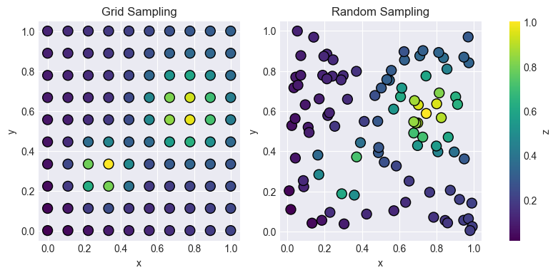
Sampling gives us an approximative representation of the actual underlying function (in this case the double gaussian). This example demonstrates only two of the available samplers. Which sampler to use depends on your application.