Tutorial: Bayesian Optimization

This tutorial explains the example Bayesian optimization workflow in Enchanted Surrogates. The Bayesian optimization example is a synthetic test case that uses the Synthetic Double Gaussian Runner, the Synthetic Double Gaussian Parser, and an example configuration file (configs/example_bayesian_optimization_local.yaml). Make sure that when you installed enchanted-surrogates, you included the optional dependencies needed for the Bayesian Optimization Sampler.

Explanation

This Bayesian optimization example aims to solve the problem "find \(x\) that makes \(f(x)\) closest to the target value \(y_{target}\)". In this example case, \(y_{target} = 2.0\).

The example runner implements a synthetic 1D objective function defined as a linear term plus two Gaussian bumps. Note that in reality, the objective function is seldom one-dimensional or simple. The formula for the objective funtion in this example is:

\[ f(x) = a \cdot x + g_{11} \cdot \exp\left(-\frac{(x - g_{13})^{2}}{g_{12}}\right) + g_{21} \cdot \exp\left(-\frac{(x - g_{23})^{2}}{g_{22}}\right) \]

The parameter values for the runner can be defined in the config file. This example uses the default parameters:

\(a = 0.2\) (linear slope)
\(g_{11} = 1.0, g_{12} = 0.001, g_{13} = 0.2\) (first Gaussian)
\(g_{21} = 0.6, g_{22} = 0.01, g_{23} = 0.7\) (second Gaussian)

The search space (bounds) for \(x\), the number of samples (budget) and the aquisition function are defined in the sampler section of the config file.

samplers:
  s1:
    type: BayesianOptimizationSampler
    budget: 50
    bounds: [[0.001, 1.0]]
    parameters: ['x']
    initial_samples: 3
    acquisition_function: LEI
    random_fraction: 0.5

In this example, the sampler starts by generating three initial_samples. These are three random points in the search space that serves are starting points for the optimization task.

Each sample is passed to the runner, which evaluates the objective function \(f(x_{sample})\). The samples and objective function evaluations (output) are passed to the parser. The parser scores each sample by how close output is to the target 2.0. In this case, the parser computes a simple distance metric:

\[ d = y_{target} - f(x_{sample}) \]

The combined run inputs and outputs are saved into enchanted_datapoint.csv after each run. Having some initial random samples, the Bayesian Optimization phase can start. Firstly, the parser reads the existing enchanted_datapoint.csv files so the sampler can reconstruct the objective from past runs. Secondly, a Gaussian Process model is trained on the data and the acquisition function (e.g., LEI) suggests new promising points to evaluate. These points (samples) are evaluated and saved into enchanted_datapoint.csv. The sampling and parsing is repeated until the budget is exhausted.

Run the example

You should be able to run the example without needing to edit the configuration file. You might want to change the base_run_dir in the supervisor section to another path for saving the data.

cd enchanted-surrogates/
python src/run.py -cf configs/example_bayesian_optimization_local.yaml

This example should not take more than a couple seconds to run.

Results

Load and analyze the results:

import pandas as pd
import matplotlib.pyplot as plt

def objective_function(x, model_params=None):
    """Evaluate the synthetic objective function."""
    if model_params is None:
        model_params = [0.2, 1.0, 0.001, 0.2, 0.6, 0.01, 0.7]

    a, g11, g12, g13, g21, g22, g23 = model_params

    y = a * x
    y += g11 * np.exp(-(x - g13)**2 / g12)
    y += g21 * np.exp(-(x - g23)**2 / g22)

    return y

df = pd.read_csv('path/to/data_dir/bayesian/enchanted_dataset.csv')
df_clean = df.dropna(subset=['x', 'output'])

fig, ax = plt.subplots(1, 1, figsize=(10, 5))
x_dense_plot = np.linspace(0.001, 1.0, 500)
y_dense_plot = objective_function(x_dense_plot)

ax.plot(x_dense_plot, y_dense_plot, 'b-', linewidth=2, label='Objective function', alpha=0.7)
scatter = ax.scatter(df_clean['x'], df_clean['output'], c=range(len(df_clean)), cmap='viridis', s=100, alpha=0.7, edgecolor='black', linewidth=1)
cbar = plt.colorbar(scatter, ax=ax)
cbar.set_label('Evaluation order', fontsize=10)
ax.axhline(y=2.0, color='red', linestyle='--', alpha=0.5, label='Target: y=2.0')
ax.set_xlabel('Parameter x', fontsize=11)
ax.set_ylabel('Output y', fontsize=11)

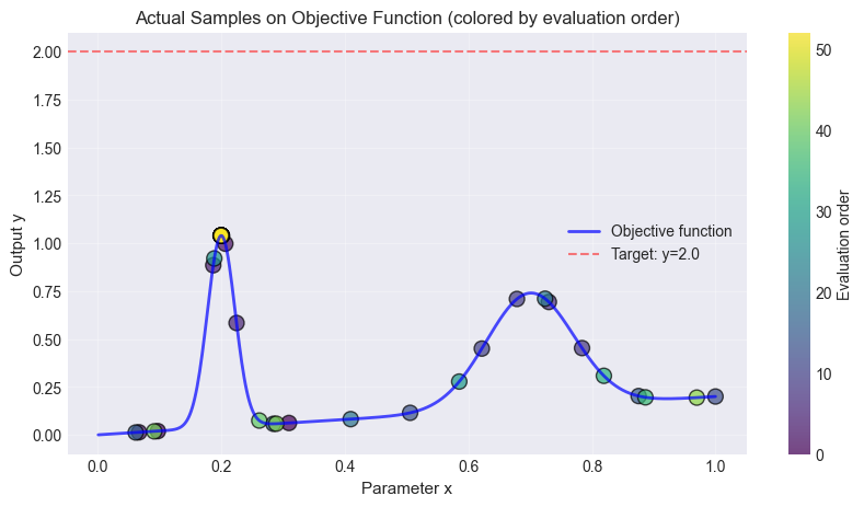
The figure below shows the objective function, the initial random points and the accuired samples. It also displays the targed \(y_{target}=2.0\) as a line. In this synthetic 1D example, it is clear that \(f(x=0.2)\) is the value closest to the target.

fig

Comparison to Pool-based Active Sampling

The same example can be ran using pool-based active sampling. The main difference is, that the pool-based active sampling will choose the best points (budget) from a pool of random candidate points (n_candidates) in order to represent the objective function. The Bayesian Optimization sampler is trying to optimize some objective (in the example above: the distance to y=2) while the pool-based active sampler is trying to find the best points to describe the underlying function.

Replace the sampler in the config file:

samplers:
  s1:
    type: ActiveLearningSampler
    bounds: [[0.001, 1.0]]
    budget: 50
    batch_size: 3
    n_candidates: 1000
    parameters: ['x']
    query_strategy: GreedySamplingTarget

Use the same plotting code as above.

fig

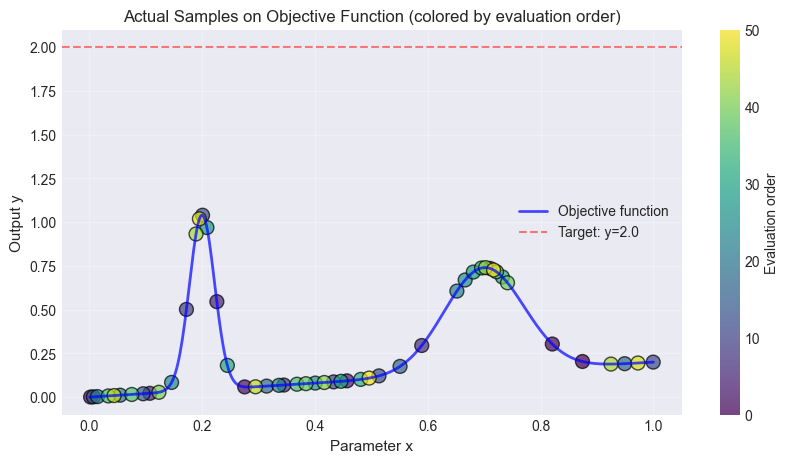
The same number of samples were taken in both examples.

Extending the example

You can adapt this example for a real simulation by:

replacing SyntheticDoubleGaussianRunner with a runner that invokes your code
implementing a parser that reads the real output files and defining your objective in collect_sample_information
updating bounds and parameters to match your input space